Exploration Risk

Risk is the probability of an undesirable outcome, usually related to monetary loss or denial of monetary gain. Frequently, we talk in terms chance of success, or the chance that the undesirable outcome does not occur. Risk of success is 1- risk of failure, if there are only two outcomes.

All hydrocarbon deposits need sufficient organic material (also called source rock), permeable formations, closure (trapping mechanism or seal) and time to form petroleum. Exploration risk analyses may include all these factors. A final factor can be lumped into the risk of "non-commerciality." This factor can come from a host of concerns- excessive drilling cost, discovery of geologically complex or highly faulted/ compartmentalized structure or a limited market for the products (gas, volatile oil, gas condensate, tar sands, kerogen). Risk factors are normally multiplied together to calculate the exploration risk, and the expected risk weighted return for investment.

A newly discovered field that tests positive for hydrocarbons may be considered uneconomic to develop. The cash flow generated from the sale of products must be sufficient to justify the investment. Non-commercial wells are considered "dry holes" under US accounting procedures.

Traps

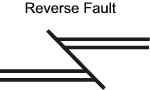
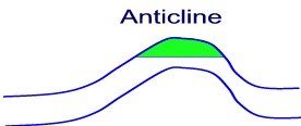
Traps may be structural, stratigraphic or a combination of these two. Growth (also normal faults) and reverse faults can be trapping mechanisms. Salt diapir (salt intrusion or salt piercement dome) is an effective trapping mechanism formed as the salt being of lighter density protrudes through layers above it. A pinchout is a form of stratigraphic trap. Also, an unconformity (missing time sequence) or an angular unconformity (tilted section is eroded, can form a stratigraphic trap. (See Wikipedia link) Anticlines is formed when the strata have bent upwards (downwards= syncline).

Salt intrusion plugs are common in the Gulf of Mexico and other field in the world. The deposits directly above plugs can be highly faulted, making for very complex structures.

Geology and Rock Properties

Additional discussion is provided in the formation evaluation section. Geologists and engineers work jointly to map out the stratigraphy of the deposits using fence diagrams. The initial evaluation stage involves intense evaluation of all petrophysical information. Commercial deposits are almost entirely either sandstone or carbonates at least at present (oil shale has a huge potential). Often sandstones are referred to as clastics, which means pieces of pre-existing rock. This makes carbonates, non-clastics. Pretty simple. One difference is that sandstone formations have depositional histories that involve transport of both organics and the sand particles. The barrier bar, deltaic marine deposits, and alluvial channel deposits all refer to sandstone deposits involving transport. In contrast, carbonate formation developed more or less their present location. For oolitic limestone, oolites are calcareous precipitates that came from the sea water. In other cases, reefs and shoals grew and subsequently, marine life lived inside the structure ultimately becoming the organic material for hydrocarbon.

The process by which deposited sediments undergo physical, chemical or biological change is referred to as diagenesis. Generally, the process decreases porosity. However, dolomitization which is the dissolution of minerals in limestone results in improved porosity. The element magnesium replaces calcium, so the density of the dolomites is increased, in the range of 2.83 to 2.87 (grain density). In some cases, dolomitization results in lower permeability, due to the placement of magnesium crystals in the pore spaces.

Sandstones and carbonates have depositional histories, resulting in properties that can vary by layer (or geological strata). Vertical permeability in sandstones may be impeded by shale breaks while in carbonates, it may be clays or other minerals. In modeling fields, many feel that the vertical to horizontal permeability ratio is generally lower in sandstone.

Once the strata is identified in the logs (SP and Gamma Ray logs are used generally), a fence diagram is drawn between wells. Structural contour maps and isopach maps further define the deposits. As the field is delineated, further mapping of the field and associated layers are needed to identify petrophysical properties.

Additional note- tapping unconventional hydrocarbon sources: Oil that has not matured sufficiently are called kerogens and the deposits referred to as oil shales, and require "cooking" or the process of pyrolysis to convert them into synthetic oils. {see Wikipedia link) . Another largely untapped resource are tar sands, which are biodegraded hydrocarbons. Coalbed methane is an unconventional gas source (see Wikipedia link).

Calculation of Oil and Gas in Place

Original oil in place is referred to the oil present at discovery. It may be abbreviated, OOIP, or OIP. It should always be referred to as the surface quantity in place. Similarly, original gas in place, can be either OGIP or GIP, and always referred to as the surface quantity in place.

Bo and Bg are Formation volume factors, and should always be expressed as reservoir volume to surface volume. Just remember it B is R before S. If there are 10 MSTB in the stock tank barrel, and Bo = 1.6, then there are 16 M rbbls were removed from the reservoir. A refers to the area of the structure in acres, porosity is expressed a fraction, and Swc is the initial or connate water saturation.

Bg and Bo can be found using correlations or from laboratory measurements (preferred). For Bg, the laboratory would identify the relationship of the Z-factor to the pressure at reservoir temperature, from which Bg can be calculated. If the Z-factor is considered to be 1, then Bg=1/p, where p is the reservoir pressure in psia.

The inverse of Bg is termed bg, and for z = 1 (ideal gas), bg = p, and this is a quick way to check if the Bg calculated is approximately correct.

In calculating in-place volumes, cutoffs may be employed, based on minimum porosity, maximum water saturation and maximum volumes of clay or shale. In these cases, it is most correct to calculate the porosity, thickness, hydrocarbon saturation product first for each log interval using the cutoffs, and then take an average of the product over the gross thickness of the oil column.

Mapping and integration of mapped values rely on computer software. See notes below on these advances.

Gas Properties

Gas properties include density, formation volume factor, gas gradients, compressibility and viscosity. Additional properties are defined later, when discussing gas-oil systems and gas condensate systems. Viscosity of gas rarely measured in the laboratory. It is obtained from the

Gas specific gravity is denoted as SG or and it is density of the gas at standard conditions (atmospheric pressure, 60 degrees F). Molecular weight of air is 28.97, so if the gas has a SG of 1.2, then the molecular weight would be 1.2*28.97. Density of gas, as presented below, is in lbs/cubic foot. For field units (degrees R, lb-mols, cu ft. and psia), the gas constant R = 10.73. As noted above, Bg is given in terms of reservoir volume to surface volume, so its units can be either Rcf/SCF or Rbbl.STB. Bg is generally less than for 1,000 psi or higher reservoir pressure. Due to the awkwardness of carrying many decimal points, some textbooks use different units for Bg. Hopefully, newer textbooks will end his practice.

The Z factor of gas is typically measured in the laboratory at reservoir temperature and for pressures ranging from atmospheric to reservoir pressure or above. Z factors can be calculated based on the composition of the gas, using the critical properties of components to calculate a pseudo-reduced pressure and temperature. Z- factors can be found in Craft and Hawkins, Figure 1.3, or Brown, K.E. Artificial Lift Methods, Vol 1. If only gas gravity is available, pseudo-critical properties are available (Figure 1.2, Craft and Hawkins) from correlations.

Gas gradients are expressed in psi/ft or . The gas gradient within a gas field are typically not significant. However, for flow up the wellbore, gas gradients will change, depending on temperature and pressures.

Gas compressibility is defined below.

Generally, these values are included in laboratory tests, or they can be easily calculated from a known z-factor verses pressure curve. In a depleting oil reservoir, gas is liberated from the oil as the pressure declines below bubble point, and with any significant gas saturation in the oil, the system compressibility can rise dramatically:

Water and oil compressibilities are on the order of 3 to 5E-6, while gas compressibility is in the 1E-3 to 1E-4 range. A 10% gas saturation can cause a 10 fold increase in system compressibility. The high compressibility of gas plays an important role in well testing and reservoir simulation. Rock compressibility can be obtained from Hall's correlation for consolidated rock. Reference 2 shows that for unconsolidated sands, rock compressibility can be considerably higher than formation compressibilities calculated from Hall's correlation. See reference 2 below.

Additional note: Software use in reservoir visualization and volumetrics

Commonly, automatic contouring programs, cross-sections and 3-D visualization software combine to provide an extended view of the field. All attributes can be mapped, which includes oil gravity, oil viscosities, net-to-gross thicknesses, oil concentrations (h*por*So) or water saturations. As the field produces, contour maps can be made of reservoir pressures (isobaric maps), water-cuts and producing gas-oil ratios. Bubble maps of produced oil, water and gas are common.

Some subjectivity exists when contouring sparce data, particularly in the extension of contours beyond control points. In this case, geological principles, existing trends, and seismic (if mapping a surface) play a role in mapping.

Software should be used in all cases to calculate reservoir volumes to remove the element of human error. In calculating reservoir volume, older books refer to the trapezoidal formula and planimeter.

References:

1. Craft, B., Hawkins, M. and Terry, R, Applied Petroleum Reservoir Engineering, 1991. Chapter 1.

2. Earlougher, R.C., Advances in Well Test Analysis, Vol 5, 1977. (See Fig D.12 on page 230, concerning rock compressibilities)

3. Allen, T.O and Roberts, A.P, Production Operations, Volume 1, Production Operations, 2006 (5th Printing).